What Is Measurement? Foundations and Philosophy of Psychological Measurement

Psychological Scale Construction

Rizqy Amelia Zein & Dian Kartika Amelia Arbi

Department of Psychology, Universitas Airlangga

2026-08-25

Outline

What are we actually doing when we “measure” something?
A short history: measurement was born of social need, not of science
Why the definition of “measurement” is still contested today
Levels of measurement (Stevens) — and the problem they leave behind
Why psychology is forced to measure indirectly
Scales, indices, and emergent variables — not every set of items is a scale
What does bad measurement actually cost?

Course orientation

What will we be doing this semester?

Final project: each group of five students will build a complete psychological scale, together with its manual.
First half (Sessions 1–7): laying the conceptual groundwork. What measurement is, which assumptions we rely on (some implicit and easy to miss), what a latent variable is, how to choose a response format, and what it means for a scale to be reliable and for scores to be valid.
Second half (Sessions 9–15): building the scale itself. Defining the construct, writing items, getting expert review, collecting pilot data, running item analysis, and developing norms and a manual.

Worth noting

The first half is not just an introduction. Almost every technical decision you will make in the second half — how many items to include, what response format to use, which coefficient to report — follows from the conceptual positions we establish in the first half.

Let us start from the most basic question

Three situations

A health psychologist wants to distinguish what patients want to happen from what they expect to happen when they see a physician. Existing scales conflate the two. She could invent a few questions herself — but what guarantees that invented questions measure anything at all?
An epidemiologist has a large national survey dataset with no stress scale in it. A handful of items seem to touch on stress. May he pool those items and call the result a “stress scale”?
A marketing team finds that parents’ purchasing decisions are driven by something they cannot name, let alone measure.

What do all three have in common?

None of them is a statistical problem. Not one is solved by choosing a fancier statistical test.
All three are measurement problems: do the numbers I produce actually stand for the attribute I claim to be studying?
And all three have the same tempting shortcut: make up the items, add them up, give it a name.

Why this matters

If you take that shortcut, every conclusion in the study rests on an assumption nobody ever checked. The problem is that the data will still look completely fine. There will still be means, still be p-values, still be a plot you can put in a paper.

The central question of this course

What makes a number

deserve to be called a measurement?

Note that this is a normative question (“deserve”), not a technical one. The answer is not inside the data.

Measurement was born before science

The earliest traces

c. 2200 BCE, China — civil service examinations for selecting officials.
A dishonest scale was treated as a moral failing, not merely a technical one — a concern that recurs across religious traditions.
- Qur’an, Al-Muttaffifin 1–3 — condemns those who demand full measure from others but give less when they weigh or measure for others.
- Qur’an, Al-An’am 152 — commands giving full measure and weight, in justice.
- Proverbs 11:1 — “A false balance is an abomination to the Lord, but a just weight is a delight.”
The French Revolution — driven in part by peasants fed up with unfair measurement practices.

What is striking about this list

Every entry is about fairness, and less about scientific accuracy. Measurement has been an instrument of power and distribution from the very beginning, something that becomes relevant again when we discuss test bias and the use of psychological tests for selection.

The idea that measurement can be wrong is relatively recent

Late 1660s: Isaac Newton, still in his twenties, appears to have been the first to average repeated observations in order to obtain a more accurate value.
But he concealed the practice for decades and did not document it in his early reports.
Why conceal it? Because at the time, discrepancies between observations were not understood as an inherent feature of measurement — they were read as evidence of incompetence.

Error and moral judgement

[17th- and early 18th-century scientists’] way of working regarded differences not as the inevitable byproducts of the measuring process itself, but as evidence of failed or inadequate skill. Error in measurement was potentially little different from faulty behavior of any kind: it could have moral consequences.

— Buchwald (2006, p. 566)

Note the gap

It took a full century after Newton before scientists widely accepted that all measurement contains error, and that averaging reduces it (Buchwald, 2006).

A conceptual shift, and the rise of psychometrics

Concealing differences between observations used to be standard practice.
- Scientists were expected to produce an “ideal picture” of a natural phenomenon, using their own judgement to decide what should count as ideal.
- As a result, “accidental” or random deviations were typically excluded from the scientific record (Daston & Galison, 2007).
The consequence of this shift was enormous: error, once read as evidence of an observer’s incompetence, came to be understood as a “systematic” — but random (stochastic) — property of the measurement process itself, one that could be modelled and estimated.
Without this shift, Classical Test Theory could not exist as we know it today.

From error to statistics

1660s, John Graunt compiled birth and death rates from christening and burial records in London, England. He averaged them to capture a “true” value he believed lay hidden behind the unpredictable events of any given year.
1777, Daniel Bernoulli compared the distribution of astronomical observations to an archer’s arrows: clustering around a central point, with progressively fewer at greater distances from it.
Buchwald (2006) argues the fundamental shortcoming of 18th-century thinking was the failure to distinguish random from systematic error — a distinction that only matured in the following century.

Remember this analogy

Bernoulli’s comparison describes what we will later call random error, and exactly why reliability can be raised simply by adding items.

How psychometrics was born

Darwin observed and measured systematic variation across species.
His cousin Sir Francis Galton extended the systematic observation of differences to humans — chiefly concerned with the inheritance of anatomical and intellectual traits.
Karl Pearson, Galton’s junior colleague, developed the mathematical tools — including the Product-Moment Correlation Coefficient that bears his name.
Charles Spearman carried the tradition forward and set the stage for factor analysis.
Alfred Binet developed tests of mental ability in France in the early 1900s.

An inheritance that is not neutral

Many early contributors to psychometrics worked within a eugenics framework. We still use their statistical tools today, but we are not obligated to carry forward the political assumptions and consequences behind them (e.g., forced sterilization or restricted reproduction for groups deemed “inferior”, among others). Knowing this history is part of being critical about the theories we use.

When psychology was declared unmeasurable

In the late 19th century Helmholtz observed that physical attributes such as length and mass share the same mathematical structure as the positive real numbers: they can be ordered and added.
The Commission of the British Association for the Advancement of Science (appointed 1932) concluded that fundamental measurement of psychological variables was impossible — because sensory perceptions cannot be ordered or added the way length and mass can.
S. S. Stevens disagreed: strict additivity is not required. People can make reasonably consistent ratio judgements — judging one sound to be twice as loud as another, for example.
L. L. Thurstone, at almost the same moment, was building the mathematical foundations of factor analysis and applying psychophysical methods to the scaling of social stimuli.

So what is measurement?

The most-quoted definition

Measurement is the assignment of numerals to objects or events according to rules.

— S. S. Stevens (1946)

This definition is very permissive, but deliberately so. It was built so that psychological measurement would fit inside it.
The consequence: almost anything can be called measurement, as long as there is a measurement rule.

Duncan’s objection

Measurement is not only the assignment of numerals, etc. It is also the assignment of numerals in such a way as to correspond to different degrees of a quality . . . or property of some object or event.

— Duncan (1984)

What Duncan adds

A correspondence requirement. Numbers must not merely follow a rule; their structure must mirror the structure of the attribute. If A has twice as much of the attribute as B, the numbers should say so too.

Duncan compares Stevens’s definition to saying “playing the piano is striking the keys of the instrument according to some pattern” — not exactly wrong, but clearly incomplete.

A more fundamental critique: Michell

Joel Michell (2007, 2011) argues that Stevens’s definition is not merely incomplete — it obscures the real question.
On his account, genuine measurement is the estimation of the ratio of a magnitude of a quantitative attribute to a unit of the same attribute.
That definition carries an empirical precondition: the attribute being measured must actually be quantitative — it must genuinely possess additive magnitude structure.

Michell’s main critique

Whether psychological attributes (anxiety, personality, motivation) are in fact quantitative is, Michell says, an empirical question that should have been tested first — but psychology skipped it and simply assumed the answer was yes. He calls this the quantitative imperative, and calls psychometrics an instance of pathological science.

You do not have to agree with Michell

Many psychometricians do not agree, and they have serious rebuttals.
But you do have to know the objection exists, and you have to be able to state which assumption you are relying on when you add up 10 Likert items into a single score.

The stance we are training in this course

Not “reject psychometrics”, and not “swallow it whole” either. Rather: know exactly which assumptions I am borrowing, and what follows if they are wrong.

Measurement vs assessment

Measurement

The principled assignment of numbers to objects or events.

Output: a score.

Assessment

The broader activity: measurement combined with interpretation and decision-making.

Output: conclusions and actions.

Why this distinction matters for your project

What you build this semester is an instrument. But the manual you write in Session 14 is an assessment document — it must tell its user how to interpret a score, and which decisions may (and may not) be made from it.

Why psychology measures indirectly

Physics vs psychology

Physics

Mass, velocity, temperature.

Observable, quantifiable, and measurable directly with an instrument.

Units agreed internationally.

Psychology

Anxiety, personality, motivation.

Cannot be weighed or measured with a ruler.

Only inferred from other things that can be observed.

Most variables of interest to social scientists are not directly observable: beliefs, motivational states, expectancies, needs, emotions, perceptions of social roles.
So we need proxies, and that is where the problems start.

Physics uses proxies too

Blood pressure and body temperature look directly observable. What we actually observe is a column of mercury or a digital readout.
We call the height of that mercury “the temperature”, when it is merely a visible manifestation of thermal energy.
For a thermometer this shorthand is almost entirely harmless — because the link between proxy and attribute is extremely tight.

What if the link is weaker?

When the relationship between a variable and its indicator is much weaker than in the thermometer case, confusing the measure with the phenomenon it is meant to reveal can lead to conclusions that are simply wrong.

This kind of error is common

In research we almost never examine relationships between variables directly.
We examine relationships between proxies. And the observable proxy is very easily confused with the unobservable variable.
DeVellis & Thorpe note a pattern that occurs often: concluding that a construct is unimportant or a theory is inconsistent, when the real problem was the measure.

A habit worth building

Every time you read “no significant relationship was found”, ask one question: was the instrument even capable of capturing that construct?

Levels of measurement, and what they hide

Stevens’s four levels

Level	Property	Psychological example
Nominal	Categories, unordered	Sex, ethnicity, diagnosis
Ordinal	Ordered, unequal intervals	Rankings, “rarely–sometimes–often”
Interval	Equal intervals, no true zero	Temperature in °C, (allegedly) Likert scores
Ratio	Equal intervals, true zero	Reaction time, number of words recalled

Look at the right-hand column

The further down you go, the harder psychological examples become to find.

What is a true zero?

A true zero means the number zero denotes the complete absence of the attribute.
Kelvin has a true zero: 100 K really is twice 50 K. Fahrenheit does not: 100 °F is not twice as hot as 50 °F.
Now try to answer: what would “zero anxiety” mean?

Psychology has almost no ratio scales

“The total absence of depression” is not an idea with a clear meaning. Which is why a statement like “group A is twice as anxious as group B” is almost never defensible, whatever the numbers say.

The core problem

Most data in psychology

are ordinal data,

yet they are treated as if they were interval.

Let us test that claim

Look at the response format you will meet most often:

1	2	3	4	5
Strongly Disagree	Disagree	Neutral	Agree	Strongly Agree

Is the psychological distance from “Strongly Disagree” to “Disagree” really the same as from “Neutral” to “Agree”?
Is that distance the same for every respondent? For every item? In every language?
Nothing guarantees it. Yet the moment we sum item scores, we have already assumed the intervals are equal.

Another example: counting symptoms

Suppose a depression score is the number of symptoms endorsed.
Is the difference between 2 and 4 symptoms the same size — clinically, conceptually — as the difference between 4 and 6?
Arithmetically both are “2”. Psychologically, almost certainly not.

The statistical consequence is real

The parametric techniques you will use — Pearson correlation, t-tests, ANOVA, linear regression — assume interval or ratio data. Applying them to ordinal data violates that foundational assumption.

So do we stop?

No. The field does treat Likert scores as interval, and there are reasonable pragmatic arguments for doing so — especially with many items and non-extreme distributions.
What we may not do is pretend no assumption is being borrowed.

What I expect from you

In your project report, when you sum items into a total score, I want you to be able to name the assumption you are making — not simply do it because everyone does. We go deeper in Sessions 2 and 4.

Not every set of items is a scale

Three things that get confused

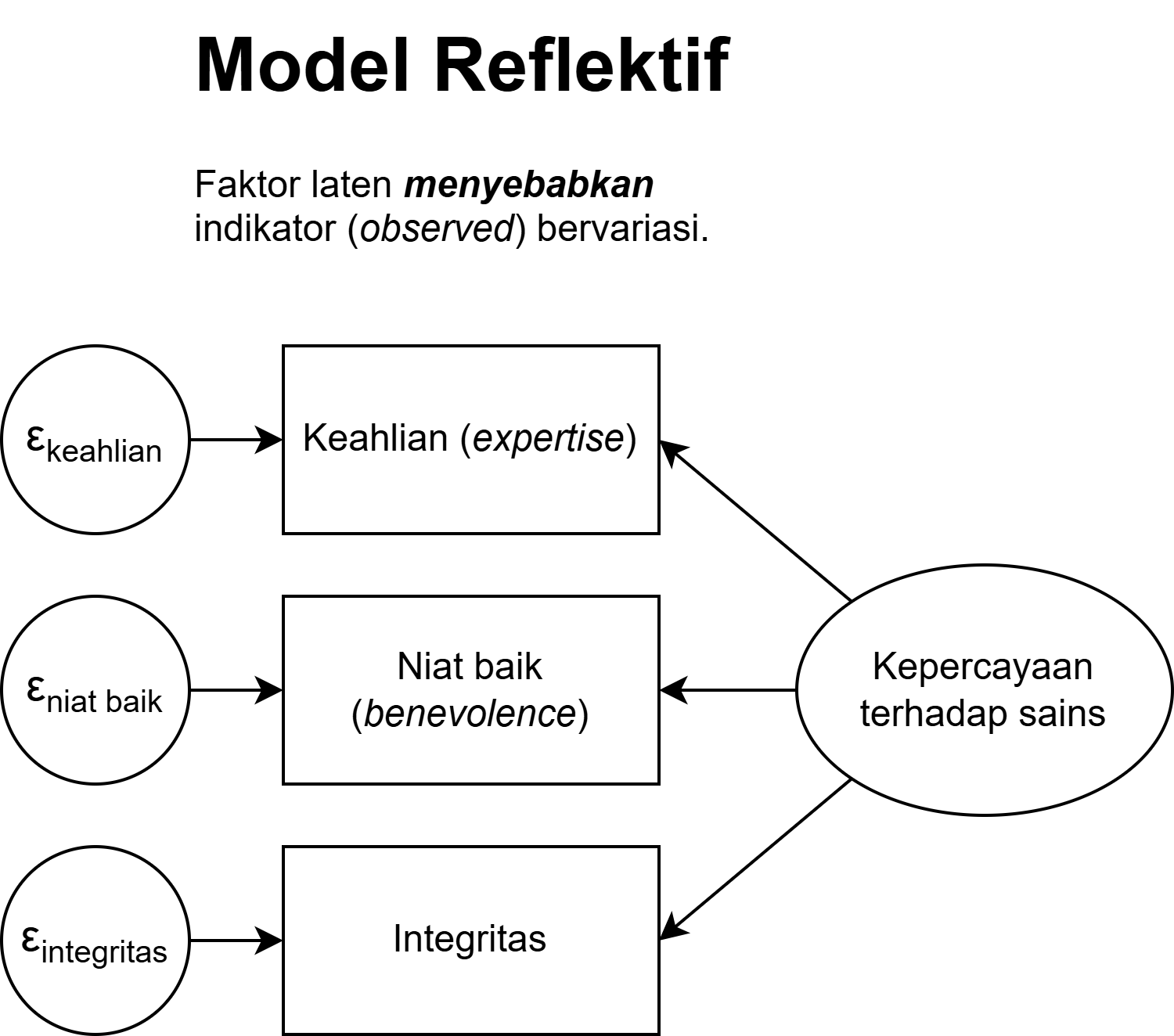
A scale — its items are effect indicators: their values are caused by the underlying construct.
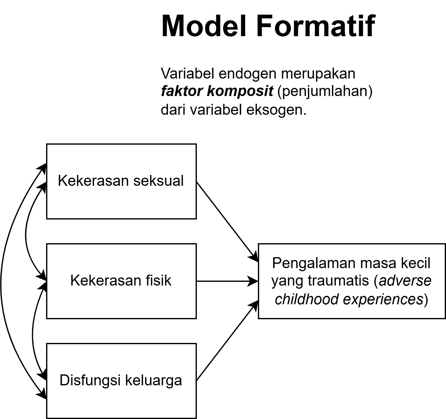
An index — its items are cause indicators: the items determine the level of the construct.
An emergent variable — a set of things grouped because someone noticed a similarity, sharing neither a common cause nor a common effect.

A scale: items as effects

Example: a measure of depression.
How someone responds to “I feel sad” and “My life is joyless” is largely determined by their affective state at the time.
The items share a common cause: that person’s depressive condition.

Practical implication

Because all items are driven by the same cause, they should correlate highly and are largely interchangeable. That is precisely what makes coefficients like \(\alpha\) and \(\omega\) sensible for a scale. Session 6.

The reflective model

An index: items as causes

Example: the electability of a presidential candidate.
Items might include: public speaking effectiveness, military service record, physical attractiveness, ability to inspire campaign workers, potential financial resources.
These characteristics share no common cause whatsoever — but they do share an effect: increasing the likelihood of a successful campaign.

A consequence that is often overlooked

In an index, items need not correlate highly and cannot be interchanged. Computing Cronbach’s alpha for an index is a conceptual error — even though the software will still print a number.

The formative model

An emergent variable: merely grouped

Sentences beginning with a word of fewer than five letters can easily be grouped together.
That group shares no common cause and no common effect. It “pops up” purely because someone — or some data-analytic program — perceived a similarity.

The warning most relevant to your project

Analysis software cannot tell these three apart. You can feed anything into jamovi and it will give you \(\alpha\), give you factors, give you a total score.

What determines whether your item set is a scale, an index, or merely an emergent variable is your theory — not the software’s output.

In summary

	Direction of causality	Items intercorrelated?	Interchangeable?
Scale	Construct → items	They should be	Yes
Index	Items → construct	Not necessarily	No
Emergent variable	Neither	Not relevant	No

What you will build this semester

A scale — with effect indicators, grounded in Classical Test Theory. But you need to know the other two exist, so that you do not mistakenly treat a genuinely formative construct as if it were reflective.

“Assembly”, not “development”

DeVellis & Thorpe observe that for many item collections, assembly is a more accurate word than development.
Researchers often throw together or dredge up items and assume the result constitutes a suitable scale.
Without ever asking whether those items share a common cause (a scale), a common consequence (an index), or merely a superordinate category (an emergent variable).

For the next 16 weeks

We are doing the development kind, not the assembly kind. That is why the process is long.

The consequences of poor measurement

There is a limit you cannot exceed

The quality of your measurement

limits the validity of the conclusions

you can draw.

Increasing your sample size, changing the statistical model, or using more sophisticated analysis will not get past this limit.

A worked example: attenuation bias

Suppose the true correlation between anxiety and procrastination is \(\rho_{T_X T_Y} = 0.60\).

You use an anxiety scale with reliability \(0.70\) and a procrastination scale with reliability \(0.65\).

The correlation you will actually observe in your data:

\[r_{XY} = \rho_{T_X T_Y} \times \sqrt{\rho_{XX'} \times \rho_{YY'}} = 0.60 \times \sqrt{0.70 \times 0.65} = \mathbf{0.40}\]

You will report 0.40 for a relationship that is really 0.60

Not because you miscalculated, and not because your sample was too small. Simply because the instruments were noisy.

Measurement and the replication crisis

Many findings in psychology fail to be replicated independently, partly attributable to imprecise measurement, combined with researcher degrees of freedom in data analysis.
Noisy measures, combined with publication bias, can actually inflate published effect sizes: only the samples that happened to produce large estimates make it into print.
Flake & Fried (2020) call this cluster of habits questionable measurement practices: not reporting how a scale was chosen, modifying a scale without saying so, not reporting its psychometric properties.

Same name, different content

Fried (2017) examined seven commonly used depression scales.
All seven claim to measure “depression”. Between them, they contain 52 different symptoms.
40% of those symptoms appear in only one scale, and just 12% appear in all seven.

What follows from this

Two studies can both report on “depression”, both use scales that are perfectly reliable, and still not be measuring the same thing. Comparing them is far more fragile than it looks.

This is the jingle fallacy: assuming two things are the same because they share a name.

The ethical dimension

Researchers often economise by using instruments that are too brief, hoping to reduce respondent burden.
But a questionnaire too short to be reliable is a bad idea, however convenient it feels.
A reliable questionnaire completed by half your respondents yields more information than an unreliable one completed by all of them.

Asking for participants’ time has ethical consequences

If the data cannot be interpreted in the end, the amount collected is irrelevant. Asking 300 people to complete an instrument that cannot possibly support a valid conclusion is an ethical problem, not merely a technical one.

Summary

Five key points

Measurement precedes science. It was born of a social need for fairness and distribution, not of scientific curiosity.
The idea that measurement contains error is only about 250 years old — and without it there would be no Classical Test Theory.
The definition of measurement is still contested. Stevens made it permissive enough for psychology to fit; Duncan and Michell argue that the permissiveness conceals an unfinished problem.
Most psychological data are ordinal but treated as interval. That is allowed — provided you know you are doing it.
Not every set of items is a scale. What decides is the direction of causality between construct and items, and that is a theoretical judgement — not a software output.

For Session 2

We will take apart the assumptions we have only touched on today:

That psychological attributes are normally distributed — where does that come from, and what supports it?
That the attribute is continuous rather than categorical.
That an item measures the same thing for every group of people.
That respondents can and will report their internal states accurately.

Preparation

Read DeVellis & Thorpe (2022), Chapter 1. If you have time, look at Chapters 1 and 2 of Petersen.

Any questions❓

Notes

These slides were built with and Quarto, using the UNAIR Theme template.
Reach me at amelia.zein@psikologi.unair.ac.id

References

Alder, K. (2002). The measure of all things. Free Press.

Bollen, K. A. (1989). Structural equations with latent variables. Wiley.

Buchwald, J. Z. (2006). Discrepant measurements and experimental knowledge in the early modern era. Archive for History of Exact Sciences, 60(6), 565–649.

DeVellis, R. F., & Thorpe, C. T. (2022). Scale development: Theory and applications (5th ed.). SAGE.

Duncan, O. D. (1984). Notes on social measurement: Historical and critical. Russell Sage Foundation.

Flake, J. K., & Fried, E. I. (2020). Measurement schmeasurement: Questionable measurement practices and how to avoid them. Advances in Methods and Practices in Psychological Science, 3(4), 456–465.

Fried, E. I. (2017). The 52 symptoms of major depression: Lack of content overlap among seven common depression scales. Journal of Affective Disorders, 208, 191–197.

Michell, J. (1997). Quantitative science and the definition of measurement in psychology. British Journal of Psychology, 88(3), 355–383.

Michell, J. (2000). Normal science, pathological science and psychometrics. Theory & Psychology, 10(5), 639–667.

Petersen, I. T. Principles of psychological assessment: With applied examples in R. https://isaactpetersen.github.io/Principles-Psychological-Assessment/

Stevens, S. S. (1946). On the theory of scales of measurement. Science, 103(2684), 677–680.